XLOOKUP: Here’s what Excel’s XLOOKUP can do
Excel’s XLOOKUP was first integrated as a beta feature in August 2019 and is currently only available in Microsoft 365 (as of July 2021). However, if you’re part of this group and regularly work with large collections of data in Excel, it is worth mastering this formula. In our tutorial, we will show some examples to explain how you can make your data search much easier with the XLOOKUP function.
What is XLOOKUP?
The XLOOKUP in Excel belongs to the family of lookup and reference functions. It is one of the most useful functions in the popular Microsoft spreadsheet software. XLOOKUP is the easiest way to search for specific data entries in a cell range. The entries in a previously defined cell range are displayed in a formatted form. Sounds familiar? This principle is also used by the VLOOKUP. However, with the more flexible Excel-XLOOKUP you can look up not only one, but several entries. It is also possible to search values vertically and horizontally in your sheet.
What does this mean in practice? Imagine you have a digital customer database as an Excel file and you are looking for the address and phone number of a certain person. With XLOOKUP you can now search for the corresponding entries by name and have the desired information displayed immediately. It doesn’t matter if the searched values are in a column, row or in a table on another page. This means that the XLOOKUP replaces not only the VLOOKUP function, but also the HLOOKUP.
XLOOKUP: Usual uses for the XLOOKUP Excel function
Before we explain the syntax of the Excel XLOOKUP function and how to use it with a few examples, here is a brief overview of the most common uses:
- Look up a single entry
- Look up multiple entries at once
- Searching rows
- Searching for exact match and next smaller or larger entries
- Using wildcard characters in the search criterion
XLOOKUP in Excel: How does the syntax work?
To work efficiently with the XLOOKUP, you should first familiarize yourself with the individual parameters. Each Excel function has a specific syntax that requires specific parameters. Even the smallest deviations can lead to an incorrect result or an error message. The following syntax applies to the XLOOKUP:
=XLOOKUP(lookup, lookup_array, return_array, [not_found], [match_mode], [search_mode])What exactly the individual parameters mean is summarized in the following table. The items with an asterisk are optional arguments in the syntax:
| Lookup | The entry you are searching for; this can be text, numbers, or wildcard characters. |
| Slookup_array | The range or array in which Excel should search for the desired information. |
| Return_array | The range or array in which you want Excel to render the desired information |
| not_found* | If Excel does not find a valid match, it may return a text or value that you provide. Otherwise, the program displays the message “#N/A”. |
| Match_mode* | The comparison mode allows you to specify a match type. |
| Search_mode* | This determines where the search should start (“1” for the first and “-1” for the last element) or start a binary search. |
Parallel to the new XLOOKUP, there is also the XMATCH function, which replaces the older MATCH-function in Excel with its improved and more expansive search functions.
XLOOKUP explained with examples
Example 1: Standard search with one return value
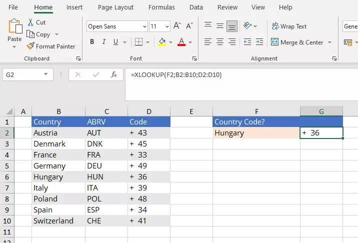
For our first example, we use only the three mandatory entries “Search criterion”, “Search mode” and “Return array”. Our Excel table has the contents in cells B2 to D10, and it maps different countries and the matching area codes. With the XLOOKUP function we now want to find out which telephone area code the country Hungary has. The result is to be displayed in area G2 (simply select the cell for this). The required formula is as follows:
=XLOOKUP(F2;B2:B10;D2:D10)F2 is the search criterion, in this case “Hungary”. The search mode consists of the prefix column and extends from B2 to B10. The return array is the column where the corresponding value is to be found, so in the example it consists of the range D2 to D10. As soon as you press the Enter key, the area code you are looking for is displayed.
You don’t want to enter the XLOOKUP in Excel by hand? Simply select the items “Formulas” and “Insert function” in the menu bar and look for the XLOOKUP in the listing. Select “All” under “Select Category” if you don’t find an entry at first.
Example 2: Standard search
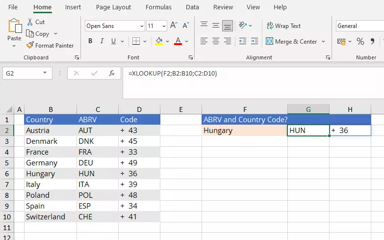
In this example, Excel outputs the area code and also the corresponding abbreviation of the selected country via XLOOKUP. For this purpose, the return array must be extended so that Excel can find both results:
=XLOOKUP(F2;B2:B10;C2:D10)If there are exact matches in the table, the XLOOKUP function will display only one of the matches. To avoid incorrect results, you can remove duplicates before your search using the function in Excel to remove duplicates.
Example 3: Search with [not_found]
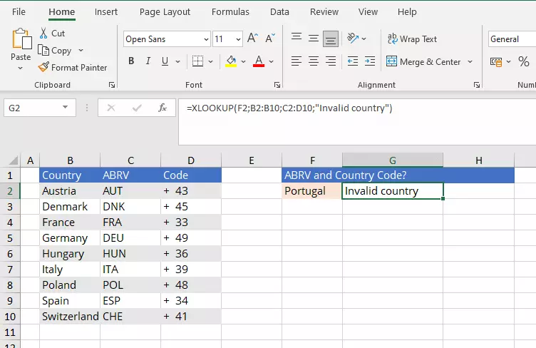
The formula in our next example contains not only the three syntax items mentioned above, but also not_found. With this addition you can specify which text should be ejected in case of a mismatch. For the example we define the text: “Invalid country” as output text and search for the country “Portugal”, which is not part of our Excel dataset.
=XLOOKUP(F2;B2:B10;C2:D10;"Invalid country")Example 4: Search with three ‘optional’ syntax
In this example, we’ll use the optional arguments not_found, match mode and search mode in addition to the three mandatory arguments.
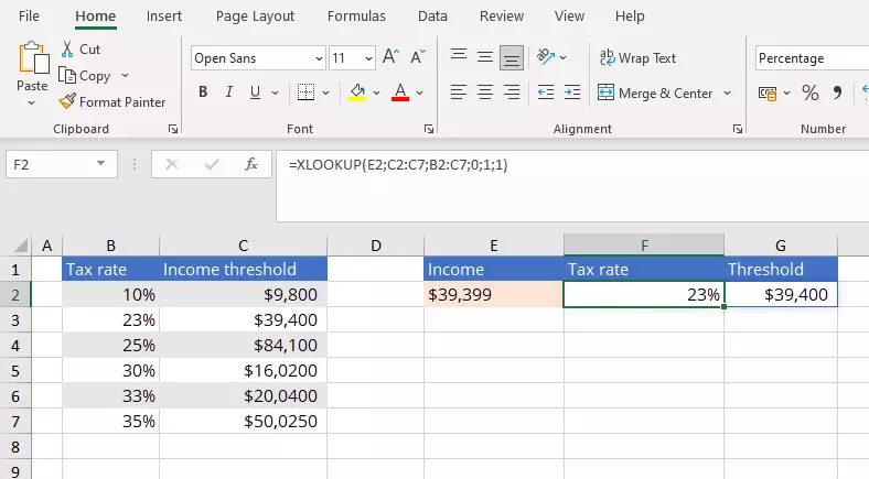
In the example table, we’re working with different tax rates and their corresponding income limits for this purpose. Using the appropriate XLOOKUP formula, we want to have the correct tax rate presented in F2 after entering the income of an employee in cell E2.
=XLOOKUP(E2;C2:C7;B2:B7;0;1;1)For not_found we have specified the value “0” in this case. So, in case of a non-match, “0” will be displayed instead of “#/NA”. Since you are not looking for an exact match, the value “1” is set for the compare mode, which means so that the next largest element is displayed. The search mode is also set to “1” so that Excel searches the table from the first to the last element.
Example 5: Nested XLOOKUP function
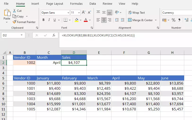
Finally, we use a nested Excel XLOOKUP function. This offers the possibility to perform a vertical and horizontal match at the same time - the real feature that makes the XLOOKUP. In the example, we are looking for the sales of the salesperson with ID “1002” in the month of April. The formula is as follows:
=XLOOKUP(B2;B6:B11;XLOOKUP(C2;C5:H5;C6:H11))If you don’t want the formula to change when you copy it, just set an absolute cell reference by putting a dollar sign ($) in front of the column and row specification.


