Excel: What can you do with the SUMPRODUCT function?
The name is admittedly somewhat misleading. The function does not give the product (result of a multiplication) of multiple sums (result of an addition). Instead, the function does the opposite: it aggregates multiple products to form a total. In Excel, SUMPRODUCT helps with everything from small tables to huge matrices.
How does the SUMPRODUCT function work?
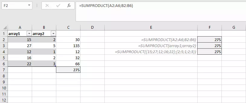
Whenever you want to multiply several values in Excel and then aggregate the results, the SUMPRODUCT function is ideal. For example, if you have several matrices in your worksheet and you want to add them together, it’s very easy to do so with SUMPRODUCT. Let’s assume we have a table with two columns: SUMPRODUCT lets you multiply the two values in each row with one another and then sum them.
SUMPRODUCT is a matrix formula. Typically, if you want to use a function as a matrix formula, you have to confirm entry of the formula using the keyboard shortcut [Ctrl] + [Shift] + [Enter]. But you don’t have to do that with SUMPRODUCT because the function is designed for processing matrices. That is why Excel doesn’t require a special command.
Syntax of SUMPRODUCT in Excel
The Excel SUMPRODUCT function has a relatively simple structure. In general, you only need to specify the range to be included in the calculation.
=SUMPRODUCT(Array1,[Array2],[Array3]...)The formula must include at least one array. You can make as many as 256 entries. Excel gives you a range of options to fill the parameters. You can enter the matrix via a cell reference, reference the required range with a name, or enter an array (a collection of values) directly in the formula.
- Cell range: =SUMPRODUCT(A2:A6,B2:B6)
- Name: =SUMPRODUCT(Array1,Array2)
- Array: =SUMPRODUCT({15,27,12,16,22},{2,5,1,2,3})
Firstly, you have to define a name for the array (e.g. “array1”) before you can use it in the function. To do so, select the corresponding range – including a header in which you have already entered the name – and then go to “Formulas and “Create from Selection”.
The corresponding cell ranges must always be symmetrical: For example, if the second array contains one row or a value less than the first range, an error message is displayed.
The SUMPRODUCT function in practice
The SUMPRODUCT function offers several advantages. The obvious advantage is that you can save several calculation steps by linking multiplication and addition. The SUMPRODUCT can also be combined with other functions. The function offers several tricks that are interesting for more complex tasks.
SUMPRODUCT with comparison
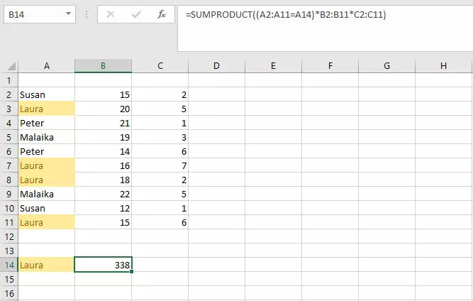
For example, SUMPRODUCT has a built-in element like the SUMIF function. It lets you choose which values in the matrices are to be added to the calculation. All you have to do is modify the actual syntax of the function somewhat:
=SUMPRODUCT((A2:A11=A14)*B2:B11*C2:C11)We have added a comparison to the first argument. The relevant cells are only multiplied and added to the total if the details correspond to the value in cell A14. Besides the equal sign that performs the comparison, multiplication signs have been added. In the normal syntax, the ranges can be separated simply using a comma. Excel often already knows how to handle the data. However, if you include a comparison, the function requires clear identification of the calculation operation. Otherwise, an error occurs.
Other multiplication options
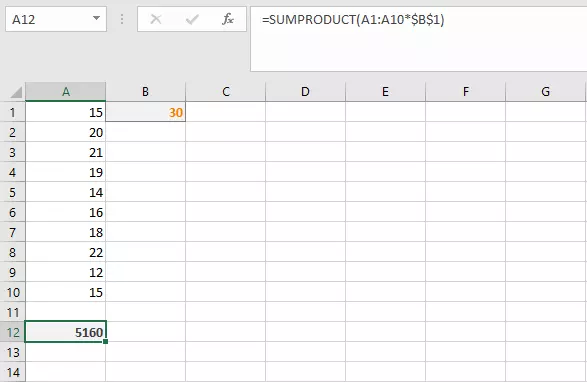
You can also use an asterisk for multiplication. As already mentioned, the function only works if the ranges specified have the same number of cells. However, you may want to multiply by the same value each time. Theoretically, you would have to use an array with the same value in every cell for this. Instead, you can enter the value just once in one row, and then use the “*” in the formula.
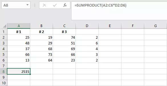
=SUMPRODUCT(A1:A10*$B$1)=SUMPRODUCT(A2:C6*D2:D6)=SUMPRODUCT((A2:A6+B2:B6+C2:C6),D2:D6)You can use the comma again in this formula. However, you have to tell Excel explicitly that you want to sum the individual ranges first.
Combining SUMPRODUCT with other functions
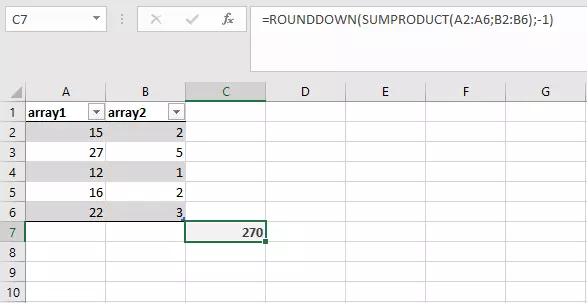
Of course, the SUMPRODUCT function can also be combined with other Excel functions. In this way, you can include multiple steps in a single formula and don’t have to use auxiliary cells to store interim results. For example, you can round the result of the function directly. Importantly, arrays will need to be of the same length for this function to work.
=ROUND(SUMPRODUCT(A2:A6,B2:B6),-1)In this example, SUMPRODUCT is nestled inside the ROUND function and serves as the first parameter.
In Excel, SUMPRODUCT can be used in numerous ways to simplify complex calculations. You can either use the function on its own or combine it with other functions.


