The Excel SUMIF function explained

Excel makes it easy to add up values in your analyses and reports. The standard SUM function is perfectly adequate in most cases. But you often want to add only specific numbers instead of adding up all the values. Excel provides the SUMIF function for this purpose.

The SUMIF function in Excel combines SUM with a logical operation. The function only sums values if they meet the criteria you specify. The criteria you specify can refer to the value itself or to a cell that refers to the value. For example, you can sum only numbers that are less than 1000. Or you can sum only the values in the “Office Supplies” category.

You can use this function to build formulas that respond to changes in your worksheets. For example, if you edit the descriptions of certain objects, they’ll no longer be included in the sum. You can also use interactive elements to develop useful forms with this function.

The syntax of SUMIF isn’t very complex.

This function has three arguments. The last one is optional:

• Range: Specify the range of cells to which you want to apply the criteria. The cells contain numbers or values. You can specify monetary values and dates. The cells can contain names, arrays or references. You can also specify the values that you ultimately want to sum.
• Criteria: You can define different types of search criteria. You can specify numbers, expressions, references, texts or other functions. If you want to use text or mathematical formulas, you have to enclose the criteria in double quotation marks. You can use wildcards ? (matches any single character) and * (matches any sequence of characters).
• Sum_range: If the values you want to sum are not already included in the first argument, you can specify them here.

If you use the optional Sum_range argument, it should contain the same number and distribution of cells as the Range argument. Each cell in the first argument is assigned one cell in the third argument. If you create a discrepancy, for example by specifying ten cells in Range but only five in Sum_range, Excel will automatically add five more cells to the third argument.

You can use the advanced function SUMIFS in addition to SUMIF. This feature is available in Excel 2007 and higher and allows you to specify multiple criteria. The principle is similar to SUMIF: You define the range that you want to search, the criteria, and the range of cells you want to sum. The main difference is that you can specify multiple criteria and select more ranges. In addition, the order of the arguments is slightly different:

Whereas the sum_range argument is optional in SUMIF, the advanced function requires you to specify the cells you want to sum. You must specify at least one criteria, define the range and you can specify up to 127 search criteria.

The Excel SUMIF function has a wide range of applications. The many possibilities of this function are best explained using examples. You can use these examples as starting points for your own projects and adapt them to your needs.

The simplest form of the SUMIF function uses logical operators. You can use the standard comparison operators in Excel:

• less than: <
• greater than: >
• less than or equal to: <=
• greater than or equal to: >=
• equal to: =
• not equal to: <>

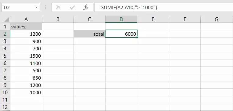
The formula adds all values in cells A2 to A10 that are greater than or equal to 1000.

SUMIF becomes even more useful when you add further cell references. For example, you can sum only those values that match a specific text in another cell.

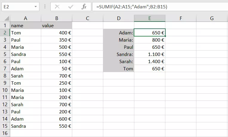
Suppose you have an unordered list of multiple deposits from different people to a savings account. You now want to see who has already transferred how much money. You can use the SUMIF function to sum only those amounts assigned to a certain name.

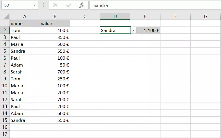
Incidentally, you don’t have to enter the text in the formula itself. You can also create a cell reference that contains the names. It can also be very useful to put the names in a drop-down list. The function then reads the search criteria from the cell.

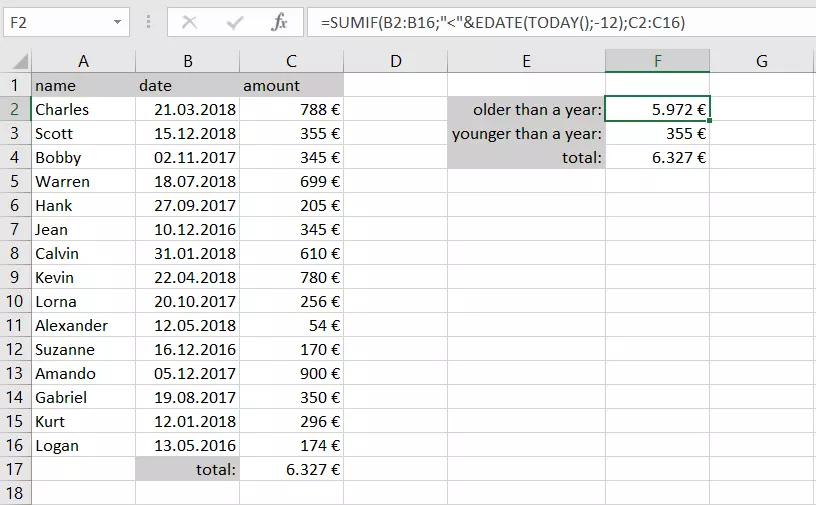
Another useful feature of SUMIF is that it can work with dates. Suppose you want to sum only those deposits that are over one year old. Once again, we’ll start with an unsorted list. You have to compare the deposit date with today’s date. To do this, use the EDATE and TODAY functions.

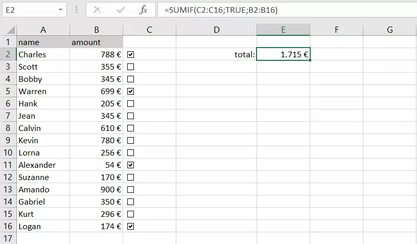
Suppose you need greater flexibility when summing values. You can also specify logical values as criteria for the SUMIF function. If the contents of the cell are TRUE, the amount in the cell is included in the sum. This can be useful if you use checkboxes, for example. Checkboxes return either TRUE (if checked) or FALSE (if unchecked) in the cell of your choice. This way your search criteria simply refers to these cells and searches for the TRUE statement in the cell.

Often you want to sum cells that meet multiple criteria. You can’t do this with SUMIF alone, so you have to use the SUMIFS function. It lets you search worksheets for two or more criteria that must be met.

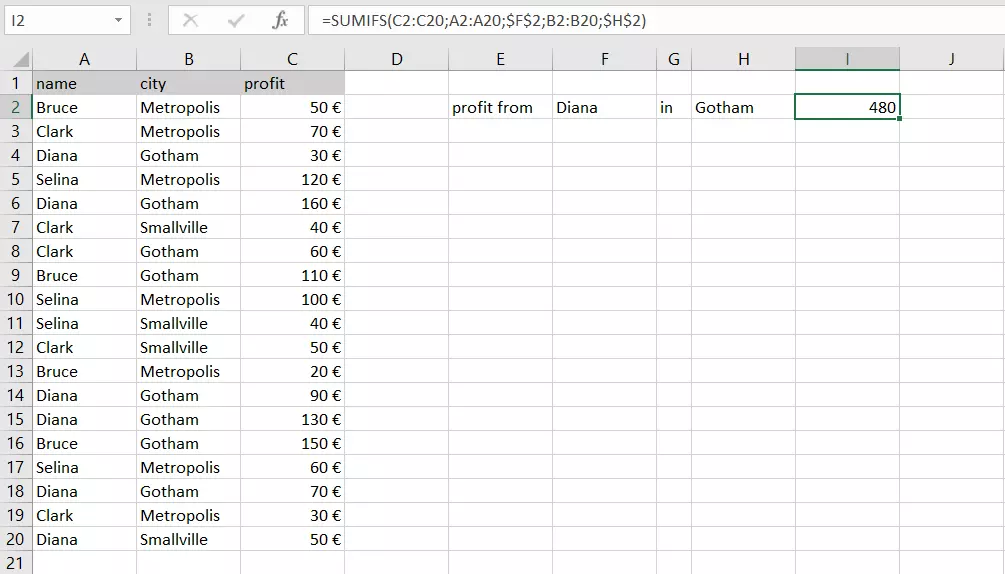
Let’s say you want to add up the profits of one of your sales reps, but only those from a particular city.