Using IFERROR function in Excel to avoid problems
The IF function is very popular for building formulas. You use it when you want Excel to do something if a certain condition is met. In most cases, the action applies to certain values or strings. But more often than you’d like, Excel displays an error message in a cell. Maybe you didn’t write the formula correctly or forgot to enter values that the formula needs in order to work properly. When this happens, you can use the IFERROR function to create an acceptable alternative.
What is IFERROR used for in Excel?
Whenever Excel is unable to perform a calculation or action correctly, the application displays an error message in the cell itself. An error message always starts with a hash sign (#).
- #NA: The formula can’t find what it’s supposed to look for.
- #VALUE!: An argument has the wrong type.
- #REF!: A formula refers to an invalid cell.
- #DIV/0!: Appears when the formula tries to divide by a cell that is either blank or has the value zero.
- #NUM!: The formula contains numeric values that aren’t valid.
- #NAME?: Usually appears when the name of a function is misspelled.
- #NULL!: Appears when you specify intersecting points that don’t actually exist.
In most cases, you respond to these errors by trying to resolve the underlying problem. But other times you might be expecting these errors and don’t want to resolve them directly. That’s where the IFERROR function comes in. It allows you to replace the displayed error value with a custom message or another value, for example.
This will keep your worksheets clearer and ensure that further calculations are not disrupted. If you’ve specified a range of cells in another formula and that range contains an error value, it’s possible that this formula will also generate an error. To avoid this situation, you can use IFERROR to enter a value so that the formula will work properly.
Excel also has an ISNUMBER function. It returns the values TRUE or FALSE depending on whether an error is found. However, most users embed it in an IF function. IFERROR eliminates the need for nested statements.
Syntax of the IFERROR function
The IFERROR function in Excel makes things very easy for you. You only have to specify two arguments: Where can an error occur? What do you want to happen if an error occurs?
=IFERROR(Value; Value_if_error)What do you specify in the arguments?
- Value: This is the argument that you want to check for an error. You can enter a calculation or other function directly, or refer to a cell.
- Value_if_error: Specify what you want to happen if an error is found. You can specify numerical values, sequences of characters or other functions. If you want to display text, it must be enclosed in double quotation marks.
Excel formulas are always preceded by an equals sign (=). If you omit it, the formula will simply appear as text in the cell. But if your actual objective is to display the equals sign in the cell, put a single quotation mark in front of the formula (').
IFERROR explained with examples
You can use this Excel function in a variety of situations, either on its own or in combination with other functions.
Alternative output with IFERROR
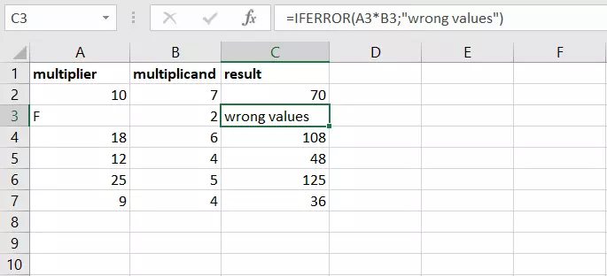
Modifying error output is probably the simplest application for IFERROR. To illustrate, let’s look at a simple calculation: The value in cell A3 is multiplied by the value in B3. If you make a typo and enter a letter instead of a number in one of the two references, Excel will return the error value #VALUE! However, you can adjust this output by linking the calculation to the IFERROR function.
=IFERROR(A3*B3; "false value")If you want to leave the cell blank in the event of an error, enter consecutive double quotation marks.
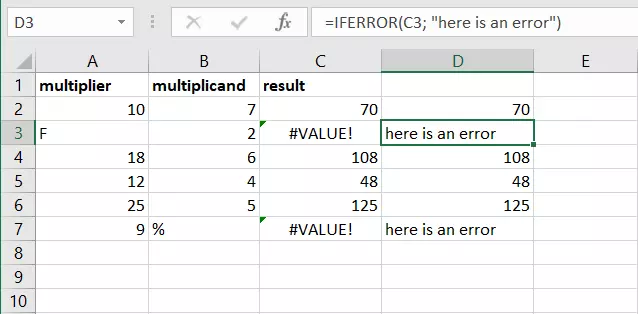
Instead of directly replacing the error message, you can apply IFERROR to another cell in order to generate a comment.
=IFERROR(C3; "Here is an error")However, if there is no error, the function displays the same value as in C2 once again. This is because the IFERROR function does not have a “Then” value. To get around this, combine IF and ISNUMBER instead:
=IF(REALERROR(C2)=TRUE; "Here is an error"; "")IFERROR & VLOOKUP: Avoiding #NV
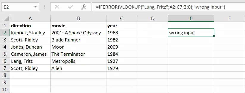
IFERROR is especially useful in combination with the VLOOKUP function in Excel. This function is well known for regularly displaying #NV errors. VLOOKUP helps you implement a search function in your Excel worksheet itself. However, if you create an error or misspell a search term, Excel will return an error message. You can use IFERROR to replace the unhelpful error value #NV with your own message.
=IFERROR(VLOOKUP("Lung, Fritz";A2:C7;2;0); "wrong input")A search for “Lung, Fritz” would generate the #NV error because the name does not appear in this spelling in the worksheet (since the last value in VLOOKUP is set to 0, no approximate values are allowed). But if you nest the function with IFERROR, your own error message will appear instead.
The IFERROR function in Excel is also helpful if you want to string together multiple VLOOKUP functions. Suppose you want to search for an object in a worksheet. If the object isn’t found, you want Excel to search the next worksheet, and so on. Since VLOOKUP generates an error when it can’t find the input, you can use IFERROR to start a new VLOOKUP.
=IFERROR(VLOOKUP(100;A3:B7;2;0); IFERROR(VLOOKUP(100;D3:E7;2;0); IFERROR(VLOOKUP(100;G3:H7;2;0); "nothing found")))Each time VLOOKUP fails to find the search string and generates an error, the function jumps to the next worksheet. If the value you’re looking for doesn’t appear in the last worksheet, a message that you specify will appear instead.
Excel also has an IFNA function. It works like IFERROR, but is limited to the error value #NA. You can use this function instead of the broader function if you only want to filter out #NA errors. All others will still be displayed. This allows you to respond better to errors in your formula.
IFERROR & SUM: Replacing errors with a value
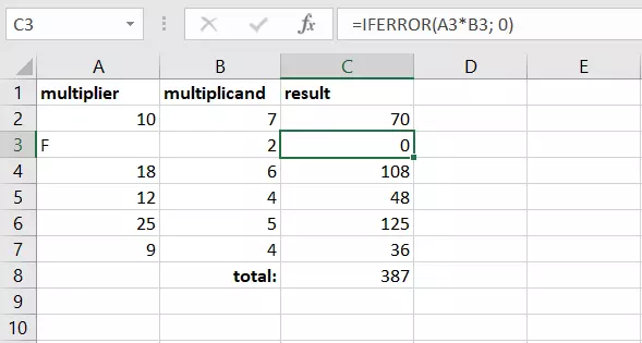
Suppose you have multiple calculations and want to add up the results using the SUM function. If you make an error in one of the calculations and Excel displays an error message instead of a numeric value, the SUM function may not work properly. Use IFERROR to protect your calculations and simply display 0 instead of the error. This way the function can perform the task and the sum won’t be distorted.
=IFERROR(A3*B3; 0)You also have the option of adding an alternative text to the SUM function simply to alert the reader to the error.
=IFERROR(SUM(C2:C7); "incorrect value")The IFERROR function allows you to replace Excel error messages with your own messages or values in a variety of situations. However, you can also use IFERROR to create complex formulas.


