How to use the IF OR formula in Excel

If you combine the Excel IF function with the OR function, it will output true even if only one of the specified conditions is true. Using simple example, we’ll explain how to use these functions together.

What is the IF OR function in Excel?

The Excel IF OR function is an extension of the popular IF formula, also known as the IF THEN function. If you combine this formula with the Excel OR function, you can define several conditions. At least one of them must be true for Excel to return the result as true. If condition A or condition B is true, condition C will be output. If neither condition is met, the formula will output condition D. The formula is structured as follows:

=IF(OR(something is TRUE,something else is TRUE),value_if_true,value_if_false)

In the formula above, the element “something is TRUE” is condition A and “something else is TRUE” is condition B. Accordingly, “value_if_true” corresponds to return value C and “value_if_false” to return value D.

Example of Excel IF OR formula

The following instructions apply to Microsoft 365 and Excel versions 2021, 2019 and 2016.

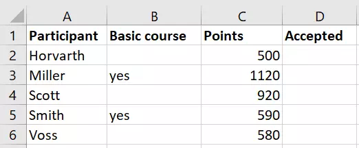
In the following spreadsheet, column A lists the potential participants for a training program. To be accepted by the institution providing the training, the individuals must have either attended a basic course or passed the entrance exam with at least 600 points.

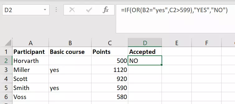
Since the conditions are already defined, we can create the formula. First, select cell D2. In this cell, the question of whether the participant should be admitted will be answered with “YES” or “NO”. The return value “YES” is output if the participant has attended the basic course (represented by the value “yes” in column B) or if the applicant scored more than 600 points on the entrance exam, which is recorded in column C. The resulting return value is “NO” if neither of the conditions have been met. Now, enter the following formula in the formula bar:

=IF(OR(B2="yes",C2>599),"YES","NO")

Once you have confirmed the formula by pressing the Enter key, Excel will display the corresponding return value in D2.

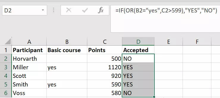
You do not need to enter the formula each time to fill in rows 3 through 6 in column D. Simply select cell D2 and drag the green rectangle to the last row. Since the formula uses a relative reference, B2 and C2 will automatically become B3 and C3 and so on.

Combining the IF OR formula with other functions

One advantage of the Excel IF OR function is that it can be combined with other useful functions. This allows you to perform more complex requests. Below you will see the spreadsheet used in the previous example. This time, both the first and last names of the potential participants are listed in columns A and B respectively.

You now want column E to display more than just the “YES” or “NO” response. You want it to output a full sentence such as “[First name] [Last name] is accepted” or “[First name] [Last name] is not accepted”. You can do this by integrating the CONCATENATE function into the IF OR function. First, select the cell range E2 to E6. Then, enter the following formula into the formula bar:

=CONCATENATE(A2," ",B2," ",IF(OR(C2="yes",D2>599),"is accepted","is not accepted"))

The first part of the formula concatenates the content of cells A and B. To prevent the individual text elements from being placed directly next to each other in the resulting return value, enter a blank space enclosed by two double quotation marks after both A2 and B2. This is then followed by the IF OR function, which completes the statement with the corresponding result.

The IF OR function in Excel can be combined with a variety of other functions. However, you should always make sure that you have used the correct number of parentheses for the nested formulas. If there isn’t a closing parenthesis, you will receive an error message. To avoid such errors, just use the formula builder under the menu option “Insert Function”, which automatically produces the correct syntax.