What is the Excel “not equal to” operator and how to use it

You can create the “not equal to” sign in Excel with two angled brackets pointing away from each other: <>. The “not equal to” sign is one of the logical operators in Excel and is used to check if values in cells differ from (don’t equal) conditions that have been specified.

What is “not equal to” used for in Excel?

In its simplest application, the “not equal to” operator determines whether or not the values in two cells are equal. The resulting output will either be TRUE or FALSE. However, the “does not equal” operator in Excel is rarely used on its own. It is often combined with functions like IF and OR to dictate what should happen when certain conditions aren’t met.

What is the syntax for the “not equal to” operator in Excel?

The simplest use of the “not equal to” sign is in a formula made up of two conditions and the “not equal to” operator:

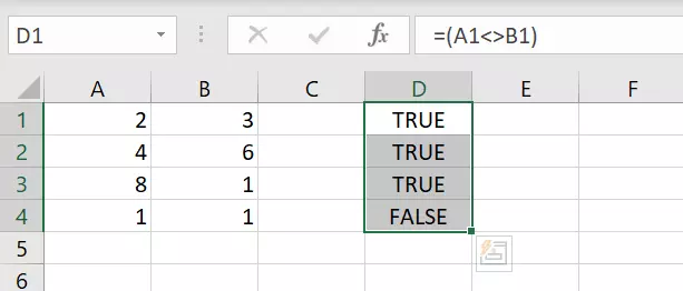
=(Condition1<>Condition2)

To illustrate this, let’s use cell A1 with the value “2” for Condition1 and cell B1 with the value “3” for Condition2. We can then use the “not equal to” operator to ask whether A1 is not equal to B1. The result is “TRUE”.

Close

You can also use “does not equal” with more than two cells, columns or values. Simply add another “does not equal” sign and another condition:

=(Condition1<>Condition2<>Condition3)

If you want to implement a “not equal to” comparison for several cells or columns, just click on the fill handle (the green square in the bottom-right corner of the cell) and pull it down to the rows you want to compare. Press Enter to implement the function with absolute reference.

Close

When using this operator in simple formulas, its implementation is rather straightforward. If you want to use it inside of a more complex formula or with a large data set though, things can get complicated. The examples used in the article should help to illustrate how the operator can be used with more complex formulas.

How to use the Excel “not equal to” operator in complex functions

Now that we’ve gone over the basic use of the “does not equal” operator, let’s take a look at how to do “does not equal” with other functions in Excel. The values that the Excel “not equal to” operator returns can help in building IF, OR and NOT functions.

Example 1: “Not equal to” + IF

The “not equal to” sign is particularly useful when combined with the IF function. The IF function asks whether certain conditions are fulfilled and if they are, the function initiates a predefined result. When implemented with IF, the “not equal to” sign is very similar to the “equals” sign.

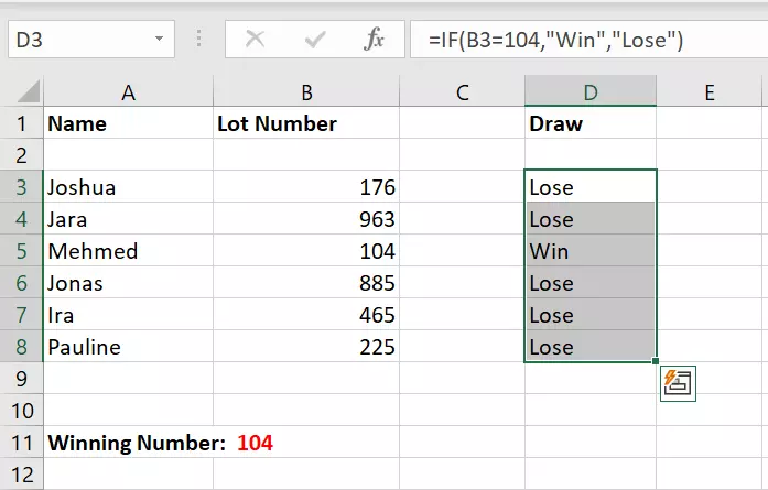
First, let’s take a look at how the “equals” operator is used together with IF. Combined with the IF function, the operator can be used, for example, to check who the winner of a raffle is by comparing the winning number to the number each person drew.

=IF(B3=104,"Win","Lose")

According to this formula, if the raffle ticket number in cell B3 is equal to the winning number “104”, then the output value will be “Win”. If it is not equal to “104”, the output value will be “Lose”. You can then use the green fill handle to apply the formula to as many cells as you need.

Close

With the “does not equal” operator, the formula will be almost exactly the same. Simply replace the EQUALS sign with the “does not equal” sign, and change the positions of “Win” and “Lose”:

=IF(B3<>104, "Lose","Win")

This formula says that if the raffle ticket number in cell B3 is not equal to the winning number “104”, then the output value will be “Lose”. If it is equal to “104”, the output value will be “Win”.

Close

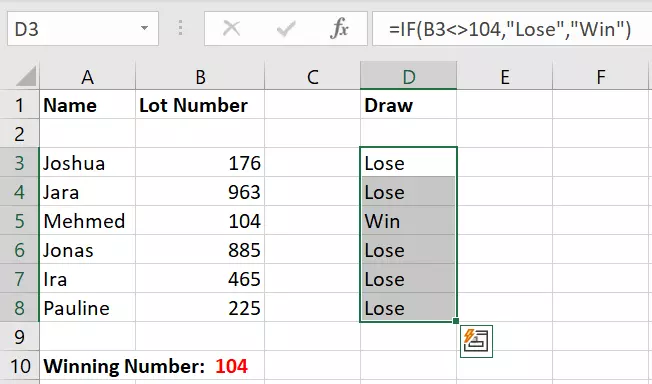
As you can see, you can get similar results with the “equals” and “not equal to” signs. As such, you can choose whichever operator is better suited to your purposes.

Example 2: “Not equal to” + IF + ODER

Once you start combining logical functions and operators, the possibilities are near endless. For example, you can combine the IF function with OR to make conditions more precise.

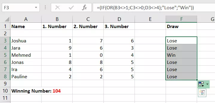
Using the raffle example, let’s take a look at how the syntax would look when we use the IF and OR functions with the “not equal to” operator:

=IF(OR(B3<>1,C3<>0,D3<>4),"LOSE","WIN")

In this case, all three of the listed numbers have to be a match in order to win. If the numbers are not equal to the winning numbers, then the output is “Lose”. Otherwise, it’s “Win”.

Close

Example 3: “Not equal to” + “SUMIF” function

The “not equal to” sign can also be useful in combination with the mathematical excel function SUMIF. SUMIF returns the sum of all the numbers that fulfill a certain condition. In the following example, SUMIF is used to add the values from cells whose adjacent cells are not empty (whose value is not equal to empty).

=SUMIF(C3:C6,"<>"&"",B3:B6)

The function will look at the values in cells C3-C6 with regard to the criterion “not equal to empty”. The function then adds the values from the cells B3-B6 for the rows that fulfill this criterion (below, rows 3 and 5). The “not equal to” sign must be put in quotations here, and then needs the & sign to combine it with the sign for empty (““).

Close

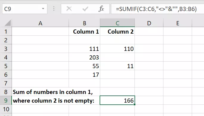
The sum of the cells in column B whose neighboring cells aren’t empty is displayed in the cell C9, which contains the formula.