How to use the Excel TRANSPOSE function
Have you tried copying from an external data source and pasting into Excel? A lot of the data is already mixed up, and by this point, you would have rather typed every single value yourself. But that doesn’t have to be the case! In addition to the simple copy function, Excel also offers the option of sorting unformatted data sets into the correct order. We explain how to transpose data in Excel.
Excel: Transposing
When you copy values from a poorly formatted data source into an Excel spreadsheet, the results may be quite useless. Instead of distributing everything neatly in rows and columns, data is, for example, continuously inserted below the last entry – with all entries in only one column. It can take a long time to subsequently sort this by hand. However, Excel also allows you to transpose data and split it into columns.
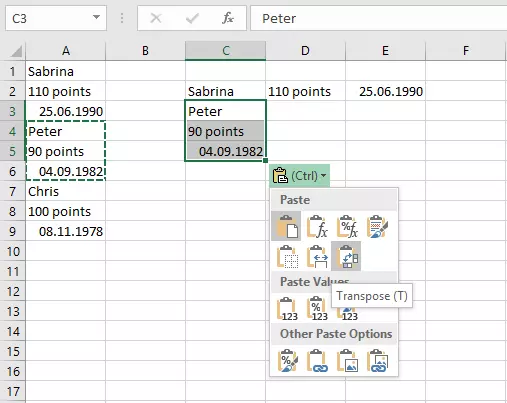
First copy a data set – i.e. all values that belong together – into the clipboard. In the Excel document, then right-click on a cell of your choice and select “Transpose”. Now the cell contents are not sorted under each other, but alongside each other. This step is repeated for all data sets and can therefore bring all the data into the desired order. This saves a fair bit of work. However, if you need to bring larger amounts of data into a new order, it is better to use formulas for this purpose.
You can also use the above technique to change the orientation of an entire table. If you copy and transpose it elsewhere, Excel automatically interchanges rows and columns. Those who reformat tables more often in this way would be better off using a pivot table.
To make things a little easier, you can also copy, paste, and transpose by using shortcuts:
- First, you mark the data area. (If the individual data sets are separated by blank rows, you can also use the combination Ctrl + Shift + *).
- Then copy the marked area with Ctrl + C.
- Navigate to the area where you want to insert the data, and then press the keyboard shortcut Ctrl + V to insert the data.
- Press 2 x Ctrl to activate the required context menu.
- With the T key, activate the transpose function.
Transpose by Formula: TRANSPOSE
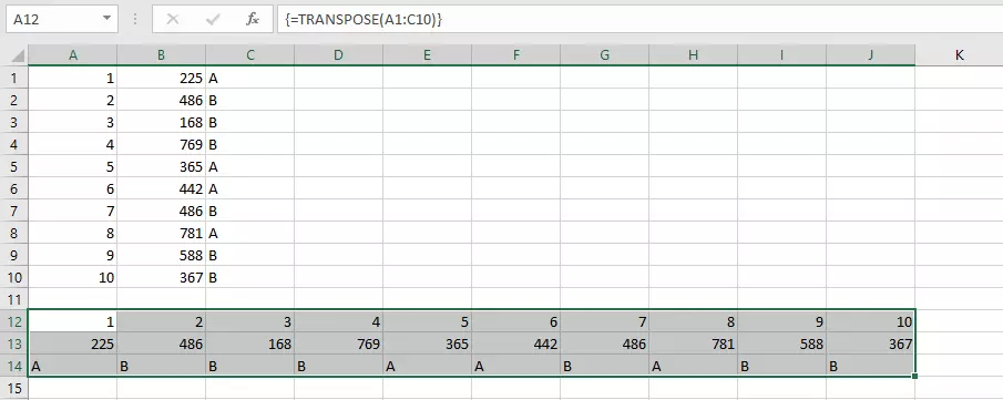
If you want to transpose data in Excel, you can also use a special function. TRANSPOSE allows you to completely re-sort a table. This is an array formula – i.e. a formula that is applied not just to one cell, but directly to several. For this, you first mark a free area that has the same size as the table that you want to transpose. If the table has 10 rows and 3 columns in its original state, select an area with 10 columns and 3 rows.
While the cells are still selected, write the TRANSPOSE function:
=TRANSPOSE(array)Array refers to the area you want to transpose. So, if the sample table is in the cells from A1 to C10 (top left cell and bottom right cell), specify the range A1:C10. The double point acts as a kind of to-sign.
The function is not confirmed – as is usual – with the Enter key. Instead, press the key combination Ctrl + Shift + Enter. Now you have a new table with the required sorting.
- Up to 50 GB Exchange email account
- Outlook Web App and collaboration tools
- Expert support & setup service


